When working with fluids, knowing what the flow field looks like is often helpful. While most experimental work is fully three dimensional, a 2D approximation will often capture the essence of the flow. In this post, I will detail how one can use the finite element library oomph-lib to “quickly” calculate the flow in almost any geometry.
This will be very quick (a few hours) if you already have oomph-lib installed and know C++ and somewhat slower if you don’t, but should work nonetheless.
The approach will be to write the geometry down in terms of polygons, read that file into the mesh generator triangle and read the resulting mesh with oomph-lib. There are already good tutorials for all these steps. This is just an example with all the steps in one place.
Set-up
I will be writing scripts in python to generate the input files for the mesh-generator. Python is generally installed on linux systems. Alternatively, you can write this file by hand if you prefer. The mesh generator triangle is freely available for download from that link. Installing oomph-lib is likely the most difficult step: detailed instructions can be found here.
Mesh-Generation
A detailed tutorial is provided by oomph-lib. My personal preference is to write a python script so I can easily modify the mesh. Let us take as an example the following geometry.

A half cylinder in a channel followed by an expansion at 45 degrees.
A quick sketch to simplify the drawing of the mesh file.

Sketch of the apparatus labelling points (A,B,C …) and boundary numbers.
I use this python script to write a poly file for the mesh generation. This is my preferred way of doing it, as I can change dimensions such as $L_{channel}$ easily.
(Aside: This script puts a set number of points onto the curved surface of the obstacle. As the elements have a node on the mid-point of each side, this will mis-represent this surface. For a more accurate representation, these mid-point nodes should be snapped to the correct position. However, this is not done in this tutorial.)
As explained in the detailed tutorial , each poly files has three parts.
Nodes:
First line: [number of vertices] [dimension (must be 2)] [number of attributes for nodes] [number of boundary markers for nodes (0 or 1)]
Following lines: [vertex index] [x] [y] [[attributes]] [[boundary marker]]
Segments:One line: [number of segments] [number of boundary markers for segments (0 or 1)]
Following lines: [segment index] [endpoint] [endpoint] [[boundary marker]]
Holes:One line: [number of holes]
Following lines: [hole index] [x] [y]
The first part of the file is a numbered list of points. The entries are the number of the point, x-position and y-position. In the second part, these points are used to defined the boundaries. Each boundary has a number, the points on the boundary and a boundary label that is used in oomph-lib. The final step is to defined holes in the domain by giving a single point that lays inside the hole. The poly file that is generated by the python script looks like this:
109 2 0 0 # of pts, 2D, no attributes or boundary markers for points
1 0.0000 -2.0000
2 0.0000 2.0000
[..]
109 12.9686 -0.9995
# END_OF_NODE_BLOCK109 1 # [number of segments (i.e. boundary edges), flag for using boundary markers here]
1 1 2 1
2 2 3 2
[..]
109 109 9 5
# END_OF_SEGMENT_BLOCK1 # [number of holes]
1 0.0000 12.5000
# END_OF_HOLE_BLOCK
This file produced by the python script, halfcylinder.poly, can the be read by the triangle mesh generator and produce a mesh with the following command:
triangle -qa1 halfcylinder.poly
The option -q sets a minimum angle of 20 degrees for all traingles and -a1 sets a maximum area of 1 for all triangles. This will generate three files: halfcylinder.1.poly, halfcylinder.1.ele, halfcylinder.1.node. These can be read into oomph-lib.
Setting the boundary conditions in oomph-lib
oomph-lib comes with a code for reading in triangle meshes. All that needs to be modified, in general, is the boundary condition. In the oomph-lib tutorial, the second example solves the Navier-Stokes equations. We have labelled the boundary in the poly file: the inflow is 1, the side walls and the obstacle are 2,4 and 5 and the outflow is boundary 3. In oomph-lib this will be shifted by one, i.e. the inflow is at boundary at 0 and the outflow is at boundary 2.
The default boundary conditions are set in the function actions_before_newton_solve(). First the minimal and maximal y-position is found, and these limits are then used to set the inflow condition on boundary 0. Otherwise, all boundary velocities are set to zero.
/// \short Update the problem specs before solve.
 /// Re-set velocity boundary conditions just to be on the safe side...
 void actions_before_newton_solve()
 {
   // Find max. and min y-coordinate at inflow
   double y_min=1.0e20;
   double y_max=-1.0e20;
   unsigned ibound=0;
   unsigned num_nod= mesh_pt()->nboundary_node(ibound);
   for (unsigned inod=0;inod < num_nod; inod++)
   {
     double y=mesh_pt()->boundary_node_pt(ibound,inod)->x(1);
     if (y > y_max)
     {
       y_max=y;
     }
     if (y < y_min)
     {
       y_min=y;
     }
   }

   // Loop over all boundaries
   for (unsigned ibound=0;ibound < mesh_pt()->nboundary();ibound++)
   {
     unsigned num_nod= mesh_pt()-> nboundary_node(ibound);
     for (unsigned inod=0;inod < num_nod;inod++)  // Parabolic horizontal flow at inflow if (ibound==0)
     {
       double y=mesh_pt()->boundary_node_pt(ibound,inod)->x(1);
       double veloc=(y-y_min)*(y_max-y);
       mesh_pt()->boundary_node_pt(ibound,inod)->set_value(0,veloc);
     }

     // Zero horizontal flow elsewhere (either as IC or otherwise)
     else
     {
       mesh_pt()->boundary_node_pt(ibound,inod)->set_value(0,0.0);
     }
     // Zero vertical flow on all boundaries
     mesh_pt()->boundary_node_pt(ibound,inod)->set_value(1,0.0);
   }
 }
 } // end_of_actions_before_newton_solve
In the problem constructor, all boundary velocities are pinned, except the horizontal part of the outflow. This ensures that the fluid leaves the device in parallel flow, without y-component, and the magnitude is set through the solutions of the equations.
 // Set the boundary conditions for this problem: All nodes are
 // free by default -- just pin the ones that have Dirichlet conditions
 // here.
 unsigned num_bound = mesh_pt()->nboundary();
 for(unsigned ibound=0;ibound < num_bound;ibound++)
 {
   unsigned num_nod= mesh_pt()->nboundary_node(ibound);
   for (unsigned inod=0;inod < num_nod;inod++)
   {
     // Pin horizontal velocity everywhere apart from pure outflow
     if ((ibound!=2))
     {
       mesh_pt()->boundary_node_pt(ibound,inod)->pin(0);
     }

     // Pin vertical velocity everywhere
     mesh_pt()->boundary_node_pt(ibound,inod)->pin(1);
   }
 } // end loop over boundaries
The default version of the code works for our case, although we are using a different geometry. This is because our inflow is on boundary 0 and our outflow is on boundary 2.
Running oomph-lib
Running the code is then a simple matter of passing the mesh files to the executable via command line arguments.
./mesh_from_triangle_navier_stokes.cc halfcylinder.1.node halfcylinder.1.ele halfcylinder.1.poly
The results are stored in the directory “RESLT”. If it has not been created, the output will fail.
Results
The output file is optimized for Tecplot. There exists a conversion script provided with oomph-lib, so that the results can be visualized using Paraview.
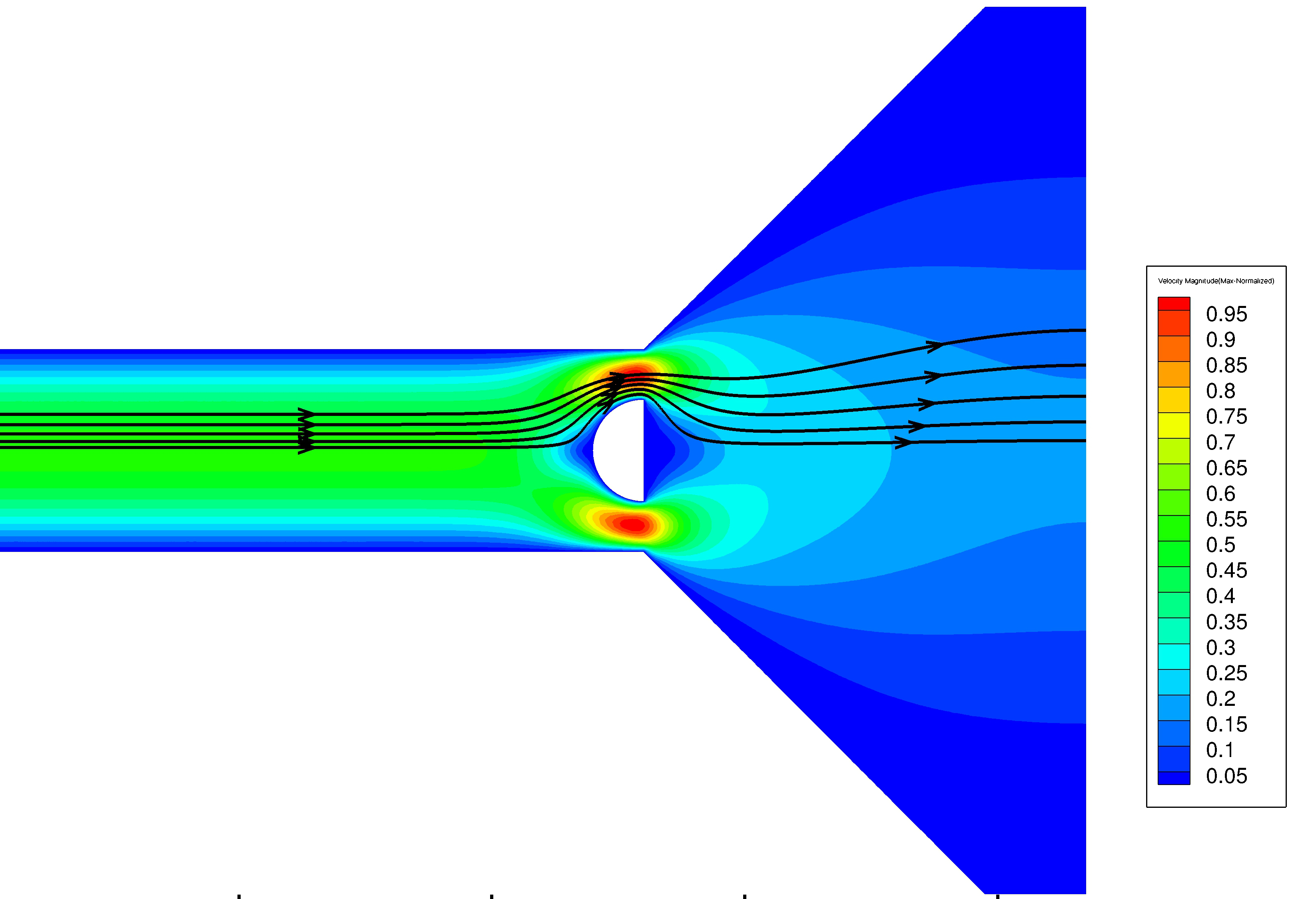
Contour plot of the speed of the fluid as well as five streamlines.
