I recently found myself in the situation where I wanted to get the trajectories of streamlines starting from a specific point. Lots of visualization software offer the possibility to plot streamlines. Two of these are Paraview and Tecplot. Paraview is open-source and generally good, although on dense meshes, streamlines tend to stop randomly. Tecplot is commercial software and I never had any problems plotting streamlines with it. However, with neither do I know how to extract streamline trajectories. If you know how to, please let me know!

In the meantime, some quick code to get streamline trajectories in Python. I am using results calculated with oomph-lib, see this earlier tutorial. The output format is optimized for Tecplot and in this example, contains 5 values: x-position, y-position, x-velocity, y-velocity and pressure. The following function will read those values from a file:

from __future__ import absolute_import, division, print_function
import numpy as np
def _read_file(path):
    '''Read output file with 5 values: x, y, u, v, p '''
    file_handle = open(path, 'r') #open file
        
    lines_list = file_handle.readlines() #read all lines
    x=[]; y=[]; u=[]; v=[]; p=[]; 
    
    for line in lines_list: #go through each line
        ent = line.split() # split into separate entries
        #ignore lines with text and those that have a different number of entries
        #the tecplot file contains zone information and information on the 
        #connectivity of each element 
        if len(ent) == 5 and ent[0][0] != 'Z': 
            x.append(float(ent[0]))
            y.append(float(ent[1]))
            u.append(float(ent[2]))
            v.append(float(ent[3]))
            p.append(float(ent[4]))
            
    return np.array(x), np.array(y), np.array(u), np.array(v), np.array(p)

The data is unstructured. This causes a bit of complication. To use the in-build python functions to e.g. plot the flow field, regularly spaced data is needed. The function scipy.interpolate.griddata thankfully does that for us.

</pre>
from __future__ import absolute_import, division, print_function
import numpy as np
from scipy.interpolate import griddata

def interpolate_data_to_uniform_grid(data, n_pts=100, plot=False):
    '''
    Approximates unstructured data with a uniform grid
    
    Input:
    data    -   a 2D numpy array with 5 columns: x, y, u, v, p
    n_pts   -   int: number of points in the uniform grid. Going above 1'000
                quickly eats GB's of RAM...
                ToDo: accept tuple for x and y dimension
    plot    -   bool: show results, mainly used for debugging
    
    Returns:
    The data interpolated on a uniform grid: xi, yi, ui, vi, pi. 
    Note that xi and yi are arrays not necessarily of equal length and a 
    value for every combination of xi and yi is returned in ui, vi and pi.
    '''
    x = data[0,:]; y = data[1,:]; u = data[2,:]; v = data[3,:];  p = data[4,:];

    # define grid.
    xi = np.linspace(np.min(x),np.max(x),n_pts*2)    
    yi = np.linspace(np.min(y),np.max(y),n_pts)
    
    # grid the data.
    ui = griddata((x, y), u, (xi[None,:], yi[:,None]), method='cubic')
    vi = griddata((x, y), v, (xi[None,:], yi[:,None]), method='cubic')
    pi = griddata((x, y), p, (xi[None,:], yi[:,None]), method='cubic')
    
    # griddata fills in NAN if it cannot fit, as is the case when outside the 
    # area of the mesh. For our purposes, zero velocity there should ensure that
    # nothing every goes there
    ui = np.nan_to_num(ui)
    vi = np.nan_to_num(vi)
    pi = np.nan_to_num(pi)

    # contour the gridded data, plotting dots at the randomly spaced data points.
    if plot:
        fig = plt.figure(figsize=(8, 6));ax = fig.add_subplot(111)
        plt.quiver(x,y,u,v,zorder=1)
        plt.axes().set_aspect('equal', 'datalim')
        plt.title("Original Data")
        
        fig = plt.figure(figsize=(8, 6));ax = fig.add_subplot(111)
        plt.quiver(xi, yi, ui, vi,zorder=1)
        plt.title("Gridded Data")
        plt.axes().set_aspect('equal', 'datalim')
        
    return np.array(xi), np.array(yi), np.array(ui), np.array(vi), np.array(pi)

Now that we have uniformly gridded data, it is easy to interpolate the velocities, using  scipy.interpolate.interp2d. We can then simply call the interpolation to get the velocity at any point in the domain. The streamlines are calculated using a simple Euler method $x_{n+1}  = x_n + u(x_n) * \delta_t$, where $x_n$ is the position at the the $n$th time-step, $u(x_n)$ the velocity at the position $x_n$ and $\delta_t$ the time-step.

from __future__ import absolute_import, division, print_function
import numpy as np
from scipy import interpolate

def get_single_streamline(xi, yi, ui, vi, start_pos, DELTAT_T=1e-3, MAX_COUNTER=1e6):
    '''Get trajectory of a streamline starting at start_pos
    
    Input:
    xi, yi, ui, vi  -    Position and velocity on a uniform grid
    start_pos       -   Tuple, x and y position of starting point
    DELTAT_T=1e-3   -   Time step used 
    MAX_COUNTER=1e10    Max number of steps
    
    Returns:
    traj_x, traj_y  -   x and y position of streamline
    
    '''  
    #normalize speed, so that the time-step means the same thing
    max_speed = np.max(np.sqrt(ui*ui + vi*vi))
    ui=ui/max_speed; vi=vi/max_speed
    
    #Interpolate the grid
    #This is somewhat doggy as we are interpolating from interpolated data.
    #This allows us to get the value of the velocities at any point.
    # A more elegant way would be to interpolate the unstructured data but this works okay.
    fui = interpolate.interp2d(xi, yi, ui, kind='cubic')
    fvi = interpolate.interp2d(xi, yi, vi, kind='cubic')
    
    #Define the dimension of our data
    MAXX=np.max(xi);MINX=np.min(xi)
    MAXY=np.max(yi);MINY=np.min(yi)

    # Now use Euler to predict the next position based on the velocity   
    traj_x=[start_pos[0]]
    traj_y=[start_pos[1]]    

    counter=0; 
    while(counter < MAX_COUNTER): 
        # Stop when we reach the edge of the domain 
        if (traj_x[-1] > MAXX or traj_x[-1] < MINX or traj_y[-1] > MAXY or traj_y[-1] < MINY):
            break;
        
        #Output to ensure the user that we are still doing something
        if counter%(MAX_COUNTER/10.0) ==0:
            print("%dth iteration" %counter)
        
        #find next position by simple euler
        xn = traj_x[-1] + fui(traj_x[-1], traj_y[-1]) * DELTAT_T
        yn = traj_y[-1] + fvi(traj_x[-1], traj_y[-1]) * DELTAT_T
        
        traj_x.append(xn); traj_y.append(yn)
        counter +=1
         
    return np.array(traj_x), np.array(traj_y)

All we need to do now is call this function to get the streamlines. An (messy) example is provided in this folder for the case considered in this tutorial. I added some functions to plot the boundaries of the domain. My aim was to get the relationship of the the $y$ position above the obstacle and the resulting angle with respect to the centreline in the expansion. In the graphs below you can see that the streamlines plotted with Tecplot show the same qualitative behaviour as those plotted with this python code.

Contour plot of the fluid speed and five streamlines. Plot produced with Tecplot.

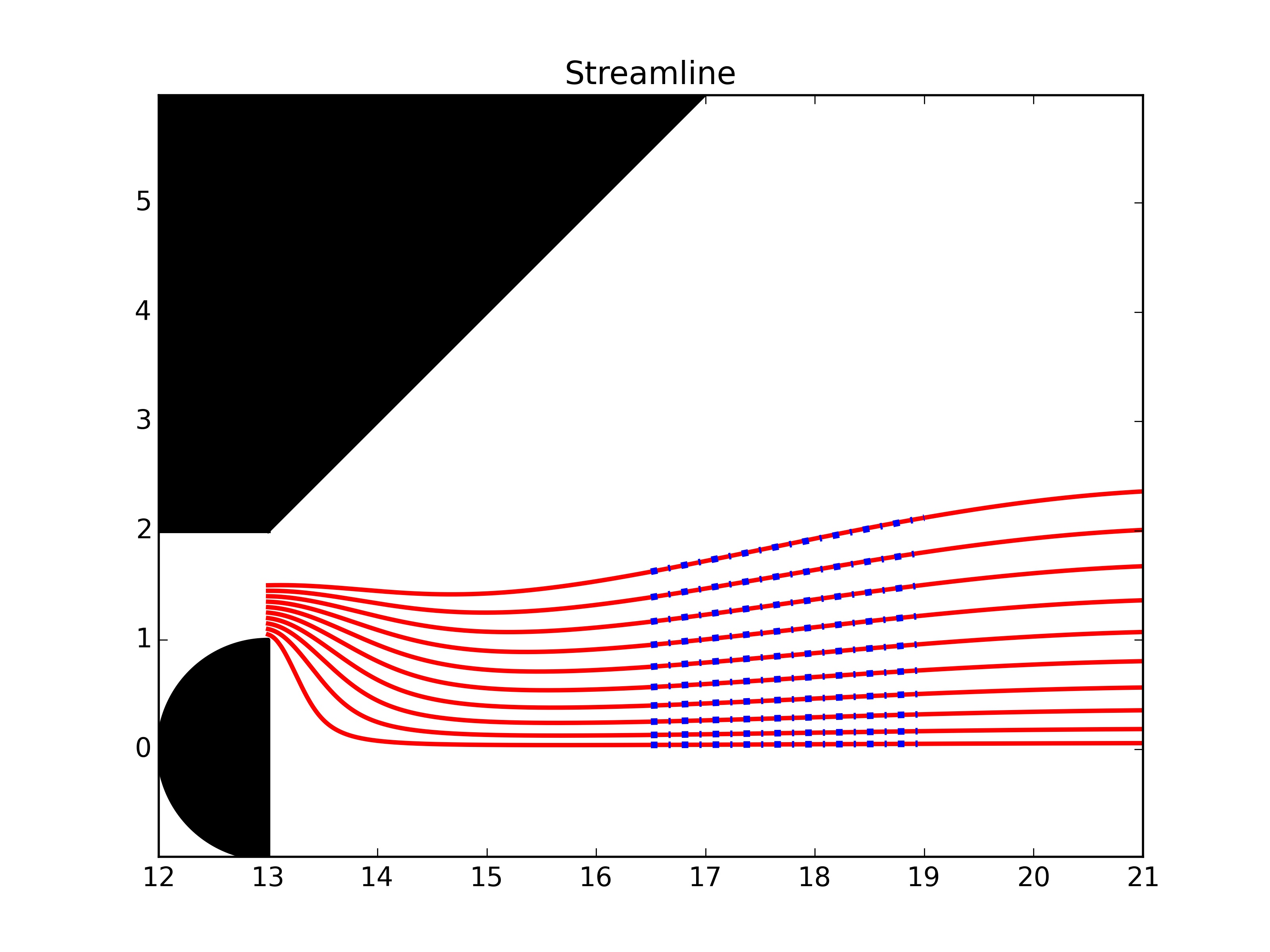
Streamlines as plotted with the python code.